What is Back-fill?
In most traditional forecasting problems like weather forecasting, data like temperatures and wind speeds from the past up to present are measured with reasonable accuracy across time and space. However in the context of COVID-19 forecasting, the current pandemic has shown a lack of similar infrastructure to produce accurate measurements of important metrics.
For example, it would be great if we knew the true COVID-19 case incidence on a daily basis. However, one major obstacle in achieving that is how testing lag tends to increase with demand, especially when a region unexpectedly becomes a hotspot without ramping up testing infrastructure beforehand.
This generally manifests in data as the phenomenon of back-fill, where measurements are retrospectively modified (as far as several months in the past). This happens when hospitals, labs and institutions take more time to process large backlogs of data with limited resources, or even when definitions change. Being able to account for uncertainty due to the back-fill process allows us to make better forecasts (or nowcasts) to assess the state of the current pandemic.
Issues and As-ofs
One of the areas I worked on at Delphi this summer was to keep track of back-fill behavior, and make it easily accessible through the COVIDcast API. Back-fill gets its name primarily from how count-based data, like number of new positive cases in a day, tends to get retrospectively “filled” or increased towards its true count, only sometimes decreasing due to rare events like false-positives or human error.
However once we start using these counts to derive other metrics like case positivity rate for the day, then the notion of “filling” no longer makes so much sense and the values simply vary. At Delphi, the more general term issue is used to refer to how a measurement can be issued multiple times. For example, the percentage of COVID-19-related doctor visits on June 1, 2020 in Kansas was retrospectively issued more than 10 times:
| geo_value | time_value | issue | value | |
|---|---|---|---|---|
| 0 | KS | 2020-06-24 | 2020-06-30 | 11.1994 |
| 1 | KS | 2020-06-24 | 2020-07-01 | 9.7082 |
| 2 | KS | 2020-06-24 | 2020-07-02 | 9.22323 |
| 3 | KS | 2020-06-24 | 2020-07-03 | 9.09493 |
| 4 | KS | 2020-06-24 | 2020-07-04 | 8.60064 |
| 5 | KS | 2020-06-24 | 2020-07-05 | 8.56377 |
| 6 | KS | 2020-06-24 | 2020-07-06 | 8.55982 |
| 7 | KS | 2020-06-24 | 2020-07-07 | 8.41921 |
| 8 | KS | 2020-06-24 | 2020-07-08 | 8.27452 |
| 9 | KS | 2020-06-24 | 2020-07-09 | 8.04732 |
This brings us to the next idea: as-of, which is really just what the data looked like as-of a certain date. Using the example above, the percentage of doctor visits in Kansas on 24 June was around 11.2% as-of 30 June, but decreased to about 8.0% as-of 9 July as more records got processed. Knowing that every data point has multiple issues, the as-of feature gives us an accurate view of what data looked like in the past, not just what it looks like now. I personally like to think of issue dates as a second dimension of time that measurements can vary over. Keeping that in mind, we normally think of a signal varying over time and space as follows:
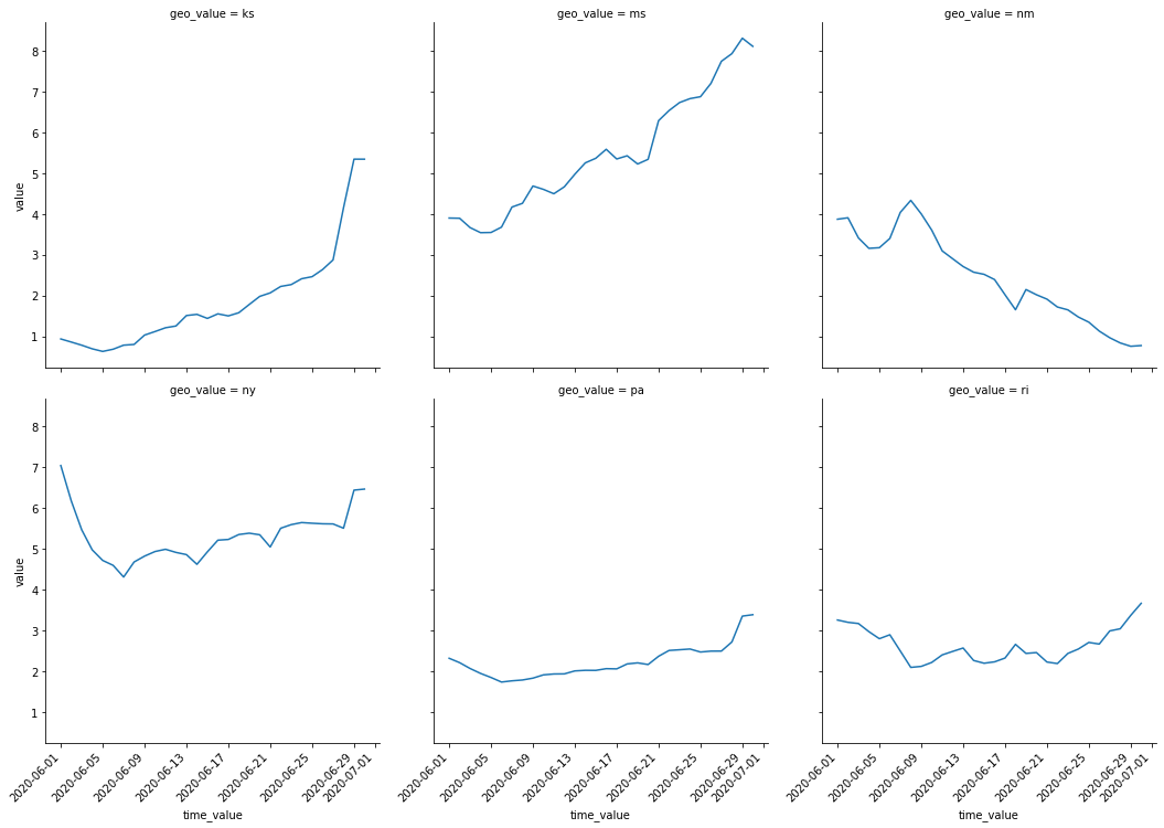
The above is a snapshot of a signal for percentage of doctor-visits related to COVID-19, as-of 7 July. But now that we know each measurement actually varied across issue dates too, what does that look like? We can also slide the as-of date across time to come up with a more nuanced visualization:
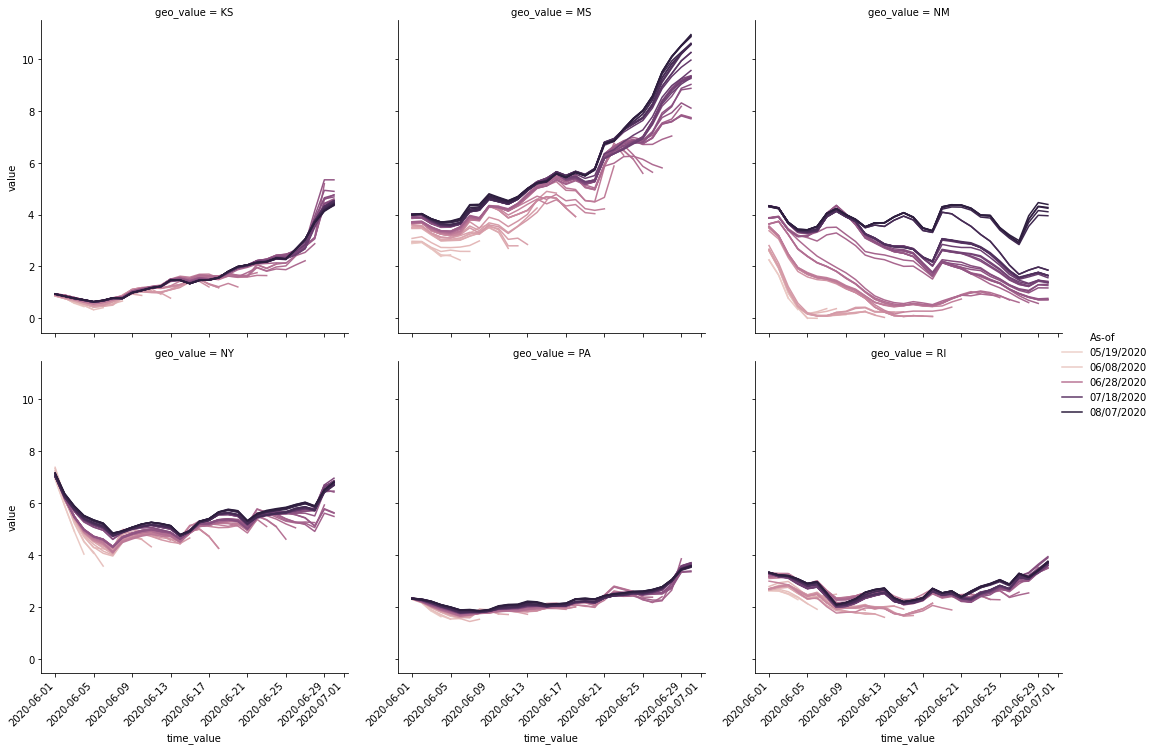
In particular, imagine you live in Mississippi and happen to find the percentage of COVID-19-related doctor visits really important. Over the month of June, you track the most recent released data every day, and you get your hopes up as it keeps seeming to trend downwards. However, if you actually waited for the back-fill / issues to roll in, you start realizing how premature that was. This brings us to the next topic, on how back-fill affects model training.
Impact on Training Models
When developing statistical models with such signals and metrics, back-fill affects modeling in at least two significant ways:
- Most-recent data probably has higher uncertainty than the less-recent ones.
- Models trained on historical data and deployed on recent data should try to match the levels of uncertainty.
The first is a direct result of how most-recent data has less issues compared to less-recent ones, as data further back in the past are more likely to most of their back-fill already rolled in. That is not to say that most-recent data is always uncertain, as back-fill is very location dependent. From the sliding-as-ofs plot before, I would be put lesser weight on recent data for Mississippi, but maybe not for Pennsylvania. Inverse-variance weighting and kernels come to mind, but actually coming up with these weights in a fair way could be tricky when we consider the second point.
The second point is a matter of matching up training and test conditions. If we naively kept track of only the latest issue of each data point, then the “historical” data has had the advantage of having its back-fill roll in till recent times. We do not get this advantage when actually trying to predict with most-recent data. Thus one has to be careful to use the right views of historical data when training, which is exactly where having a as-of view becomes useful. Train on historical data with appropriate as-of dates to match what will be done during test time!
What’s Next
A lot of work was put into the COVIDcast API to make issue dates accessible and as-of views easy to use, especially through the R and Python clients, so be sure to check it out! Code used for all examples in this post can be found in this Jupyter Notebook to play around with.
In the next post, I hope to go into technical detail about some of the challenges faced in implementing issue tracking into the COVIDcast API.
Tagged #covid19, #visualization, #data.