Graphs, Embeddings, Layouts

Recently, I got asked a pretty interesting modeling question. Given an undirected graph \(G = (V, E)\) with \(|V| = N\) vertices, can I produce embeddings of dimension \(d\) for each vertex such that:

1. Adjacent vertices have more similar embeddings
2. Non-adjacent vertices have more different embeddings

I was quite thrown off by the mentions of graphs and embeddings at first, thinking of something like a Graph Convolutional Network. However in this case, things are much simpler and there are no features associated with each vertex.

Embeddings are points in some d-dimensional space, but vertices and edges are abstract relationships with no inherent ties to coordinates. This is actually a case of a graph layout algorithm! What we really want is to find a nice assignment of coordinates to each vertex that satisfies the above conditions. For example if \(d = 2\), then this would be like a task of trying to draw out the graph on a flat surface.

I think force-directed graph drawing is a really cool approach to generating graph layouts. The graph is modeled with spring-like forces of attraction and charge-like forces of repulsion depending on adjacency. It is then run in a physical simulation to let the forces come to an equilibrium. These usually produce good-looking layouts, but could get stuck in sub-optimal layouts depending on the random initialization of positions.

In this particular case, the challenge was to formulate this as an optimization problem and solve it with something like PyTorch. The same autograd feature that makes training of deep networks declarative also makes it easy to use many flavors of gradient descent to try solve any differentiable optimization problem.

Setup

In order to use PyTorch to solve this, we need to define 3 main aspects of the optimization problem:

1. Parameters
2. Target quantity
3. Loss

Parameters

Parameters refer to the set of unknown variables we are trying to estimate, and search for through optimization like gradient descent. In this case, the unknown variables we are concerned with are the coordinates for each vertex in the graph. We shall denote the \(N\) unknown d-dimensional coordinates as the matrix \(\mathbf{X} \in \mathbb{R}^{N \times d}\).

With our gradient descent approach, we need an initial guess to the parameters to start optimizing from. A reasonable way would be to just sample some standard normals as the initial guess:

X = torch.randn((N, d), requires_grad=True)

The reason why we need requires_grad is this tells PyTorch to keep track of the computations starting from \(X\) so it can perform autograd and back-propagate to our parameters \(X\).

Target Quantity

I think there is a lot of flexibility in the target quantity, depending on how we want to solve this. I really like the physical-based approach of attraction and repulsion, and so went with that. The central quantity to this would then be the pairwise relative distance between each vertex in the graph. Once again, there could be various measures of distance like Manhattan distance, Cosine similarity, etc. But sticking to the theme of physical approaches, I chose Euclidean distance (squared). We can calculate pairwise (squared) Euclidean distances as a \(D \in \mathbb{R}^{N \times N}\) matrix as so:

diffs = X.view(1, N, d) - X.view(N, 1, d)
D = (diffs**2).sum(dim=2)

The above uses broadcasting to create an intermediate \(N \times N \times d\) tensor of the differences, \(\text{diffs}_{ijk} = x_{i,k} - x_{j,k}\). Then the pairwise Euclidean distance is \(D_{ij} = \sum_{k=1}^d \text{diffs}_{ijk}^2\).

Loss

The loss is the quantity we want to minimize in our optimization. It is the one number we use to judge how good the current parameter estimates are, where lower is better. Sticking to the theme, I chose to breakdown the loss into 3 components:

1. Attraction: \(L_{att} \propto \sum_{i, j \in Adj} D_{ij}\)
2. Repulsion: \(L_{rep} \propto \sum_{i , j \not \in Adj} \frac{1}{D_{ij}}\)
3. Centralization: \(L_{cent} \propto \sum_{i} \|x_i\|_2^2 = \|X\|_F^2\)

The first two describe the forces of attraction and repulsion, which we can say are proportional to squared distances and inverse-squared distances respectively. The third acts as a prior for our parameters, in that it reflects how I am going to prefer coordinates that are closer to the origin and penalize coordinates that are further away. This helps to address the translation invariance in possible solutions. The final loss is then \(L = \lambda_{att} L_{att} + \lambda_{rep} L_{rep} + \lambda_{cent} L_{cent}\), which lets us weight the different components separately.

eps = 1e-6

attract = (adj * dists).sum()
repel = ((1 - adj) * (1 / (dists + eps))).sum()
cent = (X**2).sum()

loss = lamb_att * attract + lamb_rep * repel + lamb_cent * cent

Results

Putting all these together, we now have defined our optimization problem in PyTorch! We can now sit back and let the autograd do the rest of the work for us:

X = torch.randn((N, d), requires_grad=True)
opt = torch.optim.Adam([X], lr=0.001)

for i in range(10000):
    opt.zero_grad()

    # Calculate squared distances
    D = ...

    # Calculate loss
    loss = ...

    # Back-propagate and optimize
    loss.backwards()
    opt.step()

Taking a step back, lets analyze what we are doing at a high level. In a force-directed approach, we are simulating a physical system of springs and charges over small timesteps and then seeing where it comes to rest. In this setup, we are instead directly searching over the parameter space for configurations of least potential energy. Our method of searching happens to be gradient descent with some learning rates.

Maybe some analogies could be drawn between how we either take derivatives wrt time or space. However, the extra features of momentum and adaptive learning rates with optimizers like Adam make it less like a true simulation and more of an optimization.

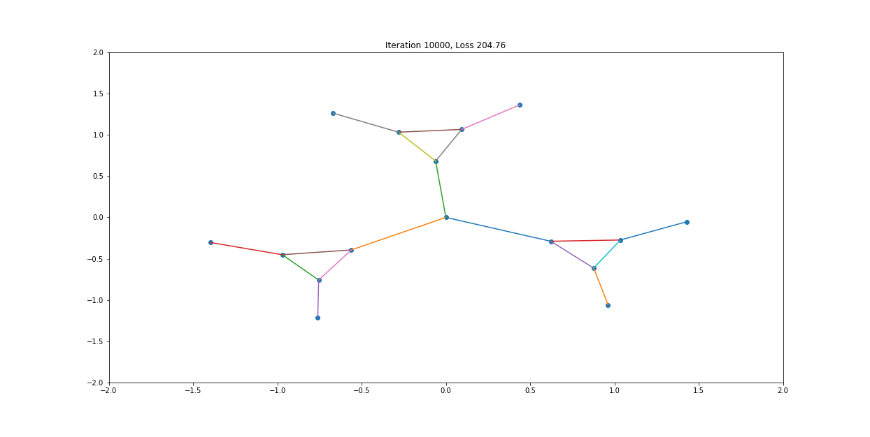
When visualized, it does happen to look like a physical simulation!

However as usual with gradient descent in non-convex optimization, we are not guaranteed to find the global optimal solution. Here is an example of the same graph with different random initializations, converging to different solutions.

As you can see, the solution on the right has a higher loss at the end, is kind of weird, and is just not a result that we would expect from this graph.

Conclusion

I thought it was quite interesting to use autograd in PyTorch to solve optimization problems outside of machine learning. Also, half of the time was actually spent generating these visualizations in matplotlib, recording them and figuring out how to make GIFs.

But also more could definitely be done to improve the aesthetic results of these embeddings. For example, running this on complete graphs would just collapse all the embeddings to the origin as every vertex is every other vertex’s neighbor. Maybe this could be solved by adding minimum distance constraints between vertices to our optimization, then converting it back into an unconstrained problem using Lagrange Multipliers.

Tagged #pytorch, #optimization, #visualization, #graphs.

---